
Data validation is a feature that allows you to control what type of data can be entered into a particular cell. It allows you to ensure that users input only valid data. In our PO form, we want to ensure the user inputs only registered items and suppliers. This helps in maintaining data integrity and accuracy in your spreadsheet. It also acts as an easier way of entering data in a form since it allows you to select values from a dropdown list.
Excel has several types of validation criteria that you can apply to cells including; whole numbers, decimal numbers, lists, dates, time, text length, and custom formulas. We will use the list option in this tutorial.
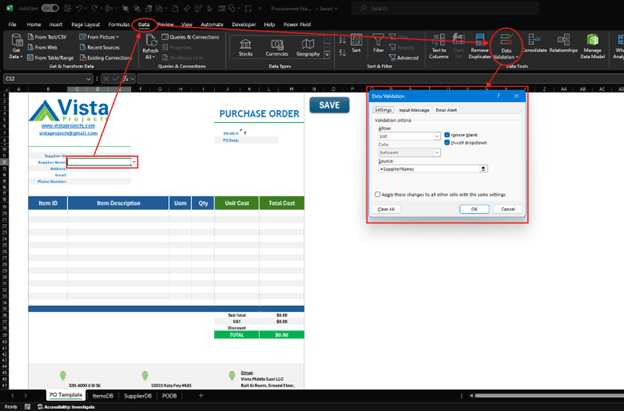
- Select the cell next to the “Supplier Name:” field.
- On the Excel ribbon, navigate to the Data tab and in the Data Tools group, select Data Validation.
- Choose the type of validation criteria (in this case list). Click inside the Source: field and press F3 on your keyboard to bring up the named ranges. Select the SupplierName and click okay.
- Highlight the entire range of cells under the Item Description column that will be used as the PO List of items. Repeat steps 2 and 3 above and choose the ItemList named range.
Once done, we are going to use XLOOKUP to get the rest of the supplier information and item information based on our selection.
How to Use the XLOOKUP Function to Get Data from Tables
The XLOOKUP Function is a powerful function that allows you to search a range or an array and returns an item that corresponds to the first match found. That is, if you have a table of 3 columns, you can search for a certain value in the first column and return it’s corresponding value in the second or third column. In our Supplier’s Table, the XLOOKUP will look for a supplier name in the Supplier Name column and return their address, phone and email address. Similarly, we will look for an item description and return its corresponding UoM, Unit Cost, and Item ID.
The XLOOKUP takes six arguments. Three arguments are required for the function to work, while the other three are optional, that is, even if you don’t include them, the function will still work.
| Argument | Description |
|---|---|
| lookup_value (required) | This is the value you want to search for |
| lookup_array (required) | The array/column/range to search |
| return_array (required) | The array/column/range from which the corresponding value will be returned. |
| [if_not_found] (optional) | Specifies what value to return if the match is not found. If omitted, Excel returns #N/A error. |
| [match_mode] (optional) | Here you define whether to perform an exact match or an appropriate match. 0 – Exact Match. If none is found, return #N/A. This is the default. -1 – Exact Match. If none is found, return the next smaller item. 1 – Exact match. If none is found, return the next larger item. 2 – A wildcard match *,?, and ~ which have special meaning. |
| [search_mode] (optional) | Specify the search mode to use: 1 – Perform a search starting at the first item. This is the default. -1 – Perform a reverse search starting at the last item. 2 – Perform a binary search that relies on lookup_array being sorted in ascending order. If not sorted, invalid results will be returned. -2 – Perform a binary search that relies on lookup_array being sorted in descending order. If not sorted, invalid results will be returned. |
For example, in order to get the address of the supplier selected in your PO template, provided you have already registered them in your SupplierDB table, here is how the XLOOKUP would look like.
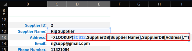
- The first argument, lookup_value, is represented by whatever will be in range C12.
- The second argument, lookup_array, is represented by, “SupplierDB[Supplier Name].” This is the syntax for referencing a table’s column inside any function/formula. The first part, “SupplierDB”, is the table name and the second part in square brackets “[Supplier Name]” is the column name.
- The third argument, return_array, is represented by “SupplierDB[Address]”. It is the same table column reference syntax as described above.
- Lastly, we tell the function to return an empty string, represented by two double quotes (“”), if a match is not found.
To get the other field values like email, phone, and ID, all we need to do is change the third argument(return_array) to reference the required column.
- SupplierDB[Email] for the Email: field
- SupplierDB[Phone] for the Phone Number: field
- SuppierDB[Supplier ID] for Supplier ID: field
The same steps used to get the Supplier information will be used to get the items information. Check out these videos for a deeper dive into XLOOKUP.
Looking for project-driven supply chain management software?
Current SCM is the first of its kind – supply chain management software purpose-built to support the most complex procurement and materials management projects. With materials management and vendor document requirements uniquely integrated into the order, Current SCM provides a unified, collaborative platform to streamline the end-to-end process of project-driven procurement and materials management.
If you are engaged in any direct procurement, technical procurement, project procurement or third-party procurement, Current SCM will improve your procurement and materials management workflow. If you are engaged in all four, Current SCM will revolutionize the way you do business.
Contact our sales professionals at Current SCM today!